8. Trees & Graphs

Trees

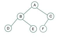
Binary Tree

A binary tree is simply a hierarchical tree that has at most 2 children for any node

A Graph would mean any number of connections for a node, and there are similarities there, but binary (2) means at most 2 children and 1 parent

class TreeNode:
    def __init__(self, val, left, right):
        self.val = val
        self.left = left
        self.right = right

Binary Tree's are both specific types of Graphs, and so are Linked Lists actually

Complete and Perfect Binary Tree

A complete binary tree is a special binary tree where all the levels of the tree are filled completely except the lowest level nodes, which are filled from the left

Complete Binary Tree

Some useful properties:

Some complete binary tree's are Perfect Binary Tree's, which means there's the maximum number of nodes at each level, but the bottom level of a complete binary tree may not be perfect
In a perfect binary tree, the number of nodes at depth $d$ is $2^d$
In a complete binary tree with $n$ nodes, the height of the tree is $\log(n + 1)$

Binary Search Tree

Binary Search Tree's are tree's who, for any node, have:

All nodes in left subtree $\lt$ node value
All nodes in right subtree $\gt$ node value

The reason these are different from regular Binary Tree's are this specific relationship - at each step you can reduce the total search space by half, resulting in $O(\log n)$ search time

The properties above ensure that there's never a grandchild node that's potentially larger than it's grandparent:

With this property ensured, we can then completely remove sub-tree's based on a current node's value:

if node.val > key:
  node = node.left
elif node.val < key:
  node = node.right
else:
  # node is val

Insertion

All new nodes are inserted as leaf nodes, and the inherent properties of BST's ensure that the tree remains valid - if we look to insert 12 into the tree below

#   10
# 8   15

def insertIntoBST(root: Optional[TreeNode], val: int) -> Optional[TreeNode]:
    if not root:
        return(TreeNode(val))
    
    if val > root.val:
        root.right = insertIntoBST(root.right, val)
    else:
        root.left = insertIntoBST(root.left, val)
    
    return(root)

insertIntoBST(root, 12)
#   10
# 8   15
#    12

Since we are forced to traverse to the end and create a new leaf node, every insertion is always $O(h)$ time complexity where $h$ is the height of the tree

Deletion

Self-Balancing Binary Search Tree

Self Balancing BST's have the same property as Binary Search Tree's, except they will balance themselves out via different methods
The reason for this balancing is that Binary Search Tree's worst case lookup time degrades to $O(n)$ $O (n)$ if the tree represents a Linked List
- This usually happens when you insert nodes in order and it becomes all right or left sides

AVL Tree

Red Black Tree

Segment Tree

Article used

A segment tree is a Binary Tree where each node represents an interval, and each node would store one or more properties of an interval that'd be queried later on

Most of the time it's segements / indexes of an array, and the total sum, count, or some aggregation over them, which allows us to find a certain aggregation over a range of data in potentially $O(\log n)$ time

LeetCode Segment Tree

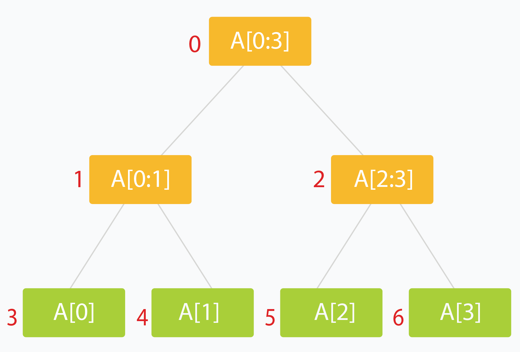
Typically the root holds the entire interval of data we're interested in traversing
Each leaf of the tree represents a range of just one single element
The internal nodes would represent the merged or unioned result of their children nodes
Ideally, each child node would represent about 1/2 of it's parent
Implementation:
- Single callable function
- Recurses down until at leaf node, and stores singular value in leaf node
- After exiting later on in recursive call merge the child values via $O(1)$ array lookup

void buildSegTree(vector<int>& arr, int treeIndex, int lo, int hi)
{
    if (lo == hi) {                 // leaf node. store value in node.
        tree[treeIndex] = arr[lo];
        return;
    }

    int mid = lo + (hi - lo) / 2;   // recurse deeper for children.
    buildSegTree(arr, 2 * treeIndex + 1, lo, mid);
    buildSegTree(arr, 2 * treeIndex + 2, mid + 1, hi);

    // merge build results
    tree[treeIndex] = merge(tree[2 * treeIndex + 1], tree[2 * treeIndex + 2]);
}

// call this method as buildSegTree(arr, 0, 0, n-1);
// Here arr[] is input array and n is its size.

The more important part is querying
- you can't read partial overlaps, it would be too confusing
- Need to traverse down until you get to a section that's smaller than your desired interval, and worst case add in from other sections as well
  - Can hopefully use some internal / middle nodes, and complete the aggregation using other leaf nodes
Updating values means finding the leaf node of the actual index, and traversing back up and out to update that leaves parents

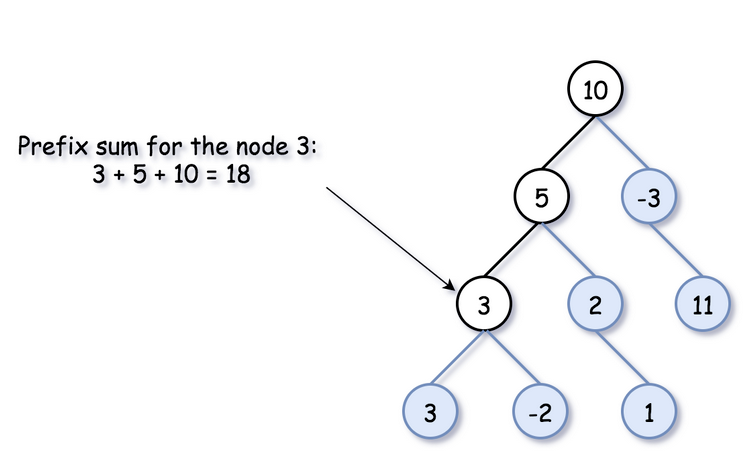
Prefix Sum

The Prefix Sum is defined, for 1-D arrays, in Arrays and Strings
The Prefix Sum also comes up in Tree Traversal because you can use it during a tree traversal technique to find things like
- Total number of paths that sum to X
- Total number of paths less than or equal to X
- etc
- The same "problems" that Prefix Sum solves for Arrays it can solve for in Trees as well

There is just one thing that is particular for the binary tree...there are two ways to go forward - to the left and to the right

To keep parent->child direction, you shouldn't blend prefix sums from the left and right subtrees in one hashmap Tree Path Prefix Sum

So to do this for Binary Tree you start off by defining some global variables

class Solution:
    def pathSum(self, root: Optional[TreeNode], targetSum: int) -> int:

    resp = 0
    target = targetSum
    freq = defaultdict(int)
    preorder(root, 0)
    return(resp)

And then you need to create the traversal code

Weird part is removing it from freq after passing, but just means you take it out so other traversals aren't affected by it, and is from Backtracking - it ensures that when you return from a recursive call (i.e., move back up the tree), the prefix sum count for the current path is removed from the frequency map

target = 3
  1
 / \
2   3

root(1) - currSum = 1, freq = {0:1, 1:1}
left to 2 - currSum = 1 + 2 = 3, freq = {0:1, 1:1, 3:1}
Done
Move back up
freq[3] -= 1 --> freq = {0:1, 1:1, 3:0}
Right to 3 - currSum = 1 + 3 = 4, freq = {0:1, 1:1, 3:0, 4:1}

Although this wouldn't affect this specific problem, with a large enough tree there'd be sums thrown all throughout here that would most likely affect the outcome

# Definition for a binary tree node.
# class TreeNode:
#     def __init__(self, val=0, left=None, right=None):
#         self.val = val
#         self.left = left
#         self.right = right
class Solution:
    def pathSum(self, root: Optional[TreeNode], targetSum: int) -> int:
        def preorder(curr: Optional[TreeNode], currSum: int) -> None:
            nonlocal resp # use the global variable

            # check existence here, not if left then left, if right then right
            if not curr:
                return
            
            currSum += curr.val
            if currSum == target:
                resp += 1

            resp += freq[currSum - target]
            freq[currSum] += 1
            preorder(curr.left, currSum)
            preorder(curr.right, currSum)

            # Remove this from map so you don't use it in other parts of tree
            freq[currSum] -= 1

        resp = 0
        target = targetSum
        freq = defaultdict(int)
        preorder(root, 0)
        return(resp)

Traversal Types

BFS explores all transformations level by level, and so the first time it reaches a node, it's *guaranteed to be the shortest path from the source node

DFS explores paths as deep as possible, and so much longer paths can be found reaching a node before the shortest one. Therefore, in scenario's where you use a seen or visited set, there's a chance you visited the node in a longer path before the shorter one, and so you'll skip over the shortest calculation

Depth First Search

Depth first search (DFS) prioritizes searching as far as possible along a single route in one direction until reaching a leaf node before considering another direction

DFS is typically only used in tree traversals, as graphs have circles and odd structures - tree's you can "go to the end" meaning a leaf node in a reasonable fashion

DFS utilizes a similar template structure to binary tree's above, but in DFS you choose what operations you do with the nodes themselves

def dfs(node):
    if node == None:
        return

    dfs(node.left)
    dfs(node.right)
    return

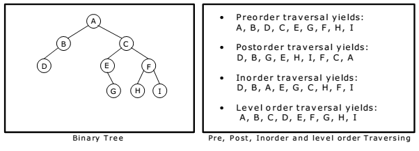
There are 3 main types of DFS, and all of them relate to where you engage with the root node:

Inorder traversal is left, root, right
Preorder traversal is root, left, right
Postorder traversal is left, right, root

def dfs(node):
    if node == None:
        return

    # operation(root) - preorder
    dfs(node.left)
    # opertaion(root) - inorder
    dfs(node.right)
    # operation(root) - postorder
    return

DFS Traversal Types

Recursion Stack

Each function call to dfs() solves and returns the answer ot the original problem (in the call stack) as if the subtree rooted at the current node was the input

Most use cases of DFS utilize recursion, and underneath the hood recursion is simply a stack

In the below tree, if we ran an inorder traversal the output would be 3, 1, 0, 4, 2, 5

    0
   / \
  1   2
 /   / \
3   4   5

def dfs(node):
    if node == None:
        return

    dfs(node.left)
    print(root) - inorder
    dfs(node.right)
    return

Looking at the call stack we would see:

call_stack = []
dfs(root) --> call_stack = [dfs(0)]
- Inside of dfs(0)
  - Call dfs(0.left) --> call_stack = [dfs(0), dfs(1)]
    - Inside of dfs(1)
      - Call dfs(1.left) --> call_stack = [dfs(0), dfs(1), dfs(3)]
        
        Inside of dfs(3)
        
        Call dfs(3.left) --> call_stack = [dfs(0), dfs(1), dfs(3), dfs(None)]
        
        Inside of dfs(None) --> return None
        
        call_stack = [dfs(0), dfs(1), dfs(3)]
        
        Call print(root) --> 3
        
        Call dfs(3.right) --> call_stack = [dfs(0), dfs(1), dfs(3), dfs(None)]
        
        Inside of dfs(None) --> return None
        
        call_stack = [dfs(0), dfs(1), dfs(3)]
        
        Exit dfs(3)
      - Call print(root) --> 1 (at this point output is 3, 1)
      - Call dfs(1.right) --> call_stack = [dfs(0), dfs(1), dfs(None)]
        
        Inside of dfs(None) --> return None
        
        call_stack = [dfs(0), dfs(1)]
And so on, and so forth!

The call_stack is just a stack that's pushe and popped to by the actual underlying python recursion, and this feature is available in basically every language. For DFS you can also implement this yourself, and it becomes an Iterable DFS solution where no recursion is involved - you simply do all of the stack calls yourself

Preorder is the cleanest implementation of this, and inorder and postorder are a bit tricky

class TreeNode:
    def __init__(self, val=0, left=None, right=None):
        self.val = val
        self.left = left
        self.right = right

class Solution:
  def maxDepth(self, root: Optional[TreeNode]) -> int:
    if not root:
      return 0

    stack = [(root, 1)]
    ans = 1

    while stack:
      curr_node, curr_depth = stack.pop()

      # preorder operation(root)
      ans = max(ans, curr_depth)

      # dfs(left)
      if curr_node.left:
        stack.append((curr_node.left, curr_depth + 1))
      # dfs(right)
      if curr_node.right:
        stack.append((curr_node.right, curr_depth + 1))      

In this way, you never leave the initial maxDepth call, and you just implement everything on a stack yourself

Time complexity - there are $n$ nodes, so we are guaranteed to do $O(n)$ work

Typically operation(root) is an $O(1)$ operation, but it may also be some other $O(k)$
If it's $O(1)$ then the entire thing is $O(n)$ , if it's $O(k)$ then $O(n \times k)$
Altogether, the time complexity is $O(n \times k)$ , where $k = 1$ is typical

Space complexity is

Usually $O(n)$ in the worst case, as you're placing all of these calls onto a stack and if the tree is straight up and down (linked list) you can reach $O(n)$
If the tree is perfectly balanced, space complexity becomes $O(\log n)$

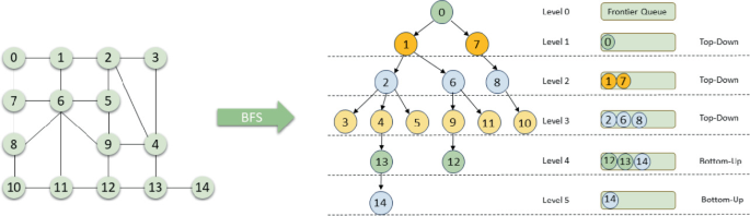
Breadth First Search

Breadth First Search (BFS) is another way to traverse tree's and graphs, but is different from DFS in that it checks row by row instead of traversing down left, right, etc depth wise

The real difference between the 2 lies in their efficiencies on problems:

BFS is better if the node is higher up, or if the logic requires level based logic
DFS is better if the node is easily found traversing depth wise, or if the logic requires it!
DFS space complexity, in typical cases, revolves around height of the tree and ends up being $O(\log n)$ , but BFS is based on the largest span of the tree, and in a perfectly balanced tree would result in $O(n)$ as the bottom row would have $n \over 2$ nodes in it
Time complexity they're usually equivalent, unless the tree structure and problem statement are weird enough to cause them to deviate
- Using underlying deque data structure is required, as using a list wil cause time complexity to explode with inserts

from collections import deque

def print_all_nodes(root):
    queue = deque([root])
    while queue:
        nodes_in_current_level = len(queue)
        # do some logic here for the current level

        for _ in range(nodes_in_current_level):
            node = queue.popleft()
            
            # do some logic here on the current node
            print(node.val)

            # put the next level onto the queue
            if node.left:
                queue.append(node.left)
            if node.right:
                queue.append(node.right)

Binary Search Tree

In a binary search tree, there's some special properties where, for any Vertex V, it's right child is greater than it's value, and its left child is less than it's value

Ultimately it's just a way to restructure a Linked List so that search is in $O(\log n)$ time - this entire concept is the idea of Self-Balancing Binary Search Trees such as B-Tree's. Self balancing tree's have less efficient writes (since they need to find where to place nodes and do some restructuring), but the idea is that reads are much more efficient

A Binary Search Tree has similar code structure to Lists

def search_bst(root, target):
    while root is not None:
        if root.val == target:
            return True
        elif target < root.val:
            root = root.left
        else:
            root = root.right
    return False

BST's follow similar time and space complexity to Binary Search, but when you traverse a BST itself you use recursion / DFS for the actual recursion, and you'd simply choose left or right instead of going down both paths

Graphs

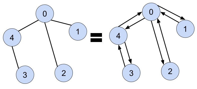
At it's core a Graph is a data structure consisting of two components - vertices (or nodes) $V$ and edges (connections between nodes) $E$

Then a Graph $G = (V, E)$ is defined by these sets of vertices and edges, both $V$ and $E$ are sets of objects

Let's say there are $n$ vertices, with $m$ edges overall, where each node can have up to $f$ features

In most production implementations the set $E$ will consist of triplets, which are objects of $(V_i, V_j, w)$ where $w$ represents the weight of the edge between vertices $V_i$ and $V_j$ . Other times it will include other information, so $(V_i, V_j, [R])$ that $R$ represents a set of relationships, but ultimately the relationships are defined by concepts such as "friends with", or "employs" or some other relationship that may or may not have weight. These features can be represented in a node feature matrix $R \in \mathbb{R}^{n \times f}$

A Graph $G$ is often stored and represented digitally using an adjacency list or adjacency matrix $A$ - then $A \in \mathbb{R}^{n \times n}$ where each node is both a row and a column, and $A[i, j]$ represents the edge between vertices $V_i$ and $V_j$

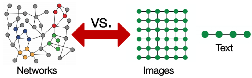
Most data structures can actually be considered specific dimensional graphs, lists are 1-dimensional graphs, trees are hierarchical graphs, images are consistently dimensioned graphs (pixel sizes), etc

Everything Is Graph

Structuring

There are 2 main ways to structure a graph in memory, either via an Adjacency List or an Adjacency Matrix

An Adjacency List is simply a list of lists, where each index represents a vertex, and the list at that index represents all of the connected vertices
- This is typically more space efficient for sparse graphs, where not every vertex is connected to every other vertex
An Adjacency Matrix is a 2-D matrix where each row and column represents a vertex, and the value at that index represents the weight of the edge between those vertices (or 1 if unweighted, or 0 if no edge)
- This is typically more space efficient for dense graphs, where many vertices are connected to many other vertices

In most real world scenarios graphs are sparse, and so Adjacency Lists are more commonly used, and even those structures are further optimized and compressed to ensure space efficiency

Representing a graph digitally is a large topic, and there are many more advanced structures like Compressed Sparse Row (CSR) or Compressed Sparse Column (CSC) formats that are used in large scale graph processing systems

For common API's on graphs we usually store 2 data structures:

Node list / set
Edge list / set

These 2 data structures allow us to traverse and manipulate the graph effectively, and are the basis for most graph algorithms - they also allow us to have heterogeneous graphs where different nodes and edges can have different types and properties. At the end of the day each of these properties typically extend an Object, so you can store any kind of data you want in them - the traversal algorithm is then expected to handle the different data types accordingly

Graph Traversal

Traversing a graph, similar to a tree, has generally 2 strategies, either Depth first or Breadth first. Separately from tree's, most graph recursive implementations need to hold onto some sort of seen = set() tracking system, similar to White / Black / Grey coloring in DFS recursion so that there isn't an infinite loop. Outside of that, the other major difference is that you don't pass node: TreeNode between dfs() calls, you have to pass node: int and use a separate data structure for storing edges, and then you traverse over those edges instead of .left or .right

Depth first means exactly as it says, from any single node you traverse as far down / as far away as you can possibly go
Breadth first on the other hand means from any node you explore each degree, or "level away", equally
- BFS is typically used in shortest path problems because as you go out a degree each level, you're guaranteed to hit the shortest path first, wheras DFS would need to search every path and then take min()
  - Although for BFS to find the optimal solution, each edge has to have equal and positve weights, and so it wouldn't work for weighted edges - that's typiaclly when you would use Djikstra's algorithm

$V$ is the number of Vertices, and $E$ is the number of edges

Operation	Time Complexity	Space Complexity
Traverse	$O(V + E)$	$O(V)$ or $O(V^2)$ if using hash map adjacency list
Traverse Fully Connected Graph	$O(V + E)$ and $E = V^2$	$O(V)$ or $O(V^2)$ if using hash map adjacency list

Graph Depth First Search

DFS involves the same data structures as mentioned above, and ultimately is the easier of the 2 to implement over graphs. The connected components example shows this, because any DFS from any node will eventually visit every node in that component, so ultimately you just use seen to track which node's you've visited so that you don't have to revisit them (infinite loop).

def dfs(start):
    stack = [start]
    while stack:
        node = stack.pop()
        for neighbor in graph[node]:
            if neighbor not in seen:
                seen.add(neighbor)
                stack.append(neighbor)

Graph Breadth First Search

Similar to tree's, both DFS and BFS can work, but usually DFS is chosen as it's easier to implement compared to BFS

Instead of levels on a tree, BFS on graphs runs at levels from a source node - at any level d, we will directly store all nodes at level d+1 next for iterating over. So BFS, in either trees or graphs, is a useful tool that's required when you need to search things based on levels deep from, or levels away from, a node. In graphs, this mostly occurs in shortest path problems, because any level would describe the shortest number of hops it has taken to reach from source node - every time you reach a node that's not in seen, you must have reached it in the minimum steps possible from wherever you started your BFS

BFS Levels

Outside of this, BFS uses the same deque data structure, and overall has a similar pattern to what it did in tree's, except you still need to check seen each time, and for the most part there is usually a maze or matrix with directions and adjacent cells we need to visit

while queue:
    row, col, steps = queue.popleft()
    if (row, col) == (n - 1, n - 1):
        return steps
    
    for dx, dy in directions:
        next_row, next_col = row + dy, col + dx
        if valid(next_row, next_col) and (next_row, next_col) not in seen:
            seen.add((next_row, next_col))
            queue.append((next_row, next_col, steps + 1))

Implicit Graphs

Similar to binary search solution space, there may be some implicit data structures that can be represented as graphs that we should check for - most occur as patterns of permutations, combinations, and choices from one inherent state to another

The time and space complexity of these problems revolves around the total number of states (nodes), and then the number of edges is usually also equal to that as you typically transition from one state to the other by tweaking one portion of the combination

Graph Problems and Advanced Data Structures

Some typical graph problems and extended data structures for solving them

Maze

Maze's are a special kind of graph where you essentially have a connected 2-D diagram

Most common examples are Finding The Nearest Exit or something similar, where you will use Breadth First Search to traverse outwards checking over the course of a structure

Connected Components

Connected Components is a way for us to find all of the clusters in a graph, where connectivity can be weak, strong, or a few other types like unilaterally

Weak connected components can be thought of as undirected connected components, so that edges are just generic edges
Strongly connected components would require directed edges between all pairs of vertices meaning there has to be a way to get to any node, NodeA, from any other node in the component NodeB
Algorithms:
Breadth First Search:
- For all nodes, start a BFS traversal as long as they aren't marked as already visited
- Traverse all neighbors $node_{j's}$ of $node_i$ , marking them as visited
- Continue the traversal until all nodes in the connected component of $node_i$ are visited
- Repeat for all unvisited nodes to find all connected components.
UnionFind above will have the root vector at the end corresponding to all of the unique connected component ID's

There are a few "typical" methods for finding connected components:

Loop over every possible node and run DFS to saturate a seen() set. Count number of dfs calls started as the number of connected components which is shown here
Utilize disjoint set union find and count the number of unique parents

Cycles + Connected Components In Undirected Graph

Undirected graphs make cycles a confusing topic - if we are traversing the graph on node 0 and we go to 4, there's going to be a neighbor in adj_list[4] that points to 0. We can remove the parent from 4's adjacency list, but it's easier just to track the original node that was used to traverse to any other node (i.e. it's parent)

Undirected Graph Cycle

Show Python Script

class Solution:
    def validTree(self, n: int, edges: List[List[int]]) -> bool:
        if len(edges) != n-1:
            return(False)
        
        neighbors = [[] for _ in range(n)]
        for e1, e2 in edges:
            neighbors[e1].append(e2)
            neighbors[e2].append(e1)

        parent = {0: -1}
        stack = [0]

        while stack:
            curr = stack.pop()
            for neighbor in neighbors[curr]:
                if neighbor == parent[curr]:
                    continue
                
                # This equates to a cycle. We want to ensure
                #   the cycle in an undirected graph of neighbors
                #   isn't tripping this up, but if we find this 
                #   node that isn't our direct neighbor / parent
                #   then it's a cycle
                if neighbor in parent:
                    return(False)
                parent[neighbor] = curr
                stack.append(neighbor)
        
        return(len(parent) == n)

There's a further invariant in graph theory: """ For the graph to be a valid tree, it must have exactly n - 1 edges. Any less, and it can't possibly be fully connected. Any more, and it has to contain cycles. Additionally, if the graph is fully connected and contains exactly n - 1 edges, it can't possibly contain a cycle, and therefore must be a tree! """

Which boils this problem down to "is the graph fully connected, and contains n-1 edges", which further boils down to "is it a single connected component with n-1 edges", which can utilize the disjoint set algorithm to check for a singular connected component, and then just count the edges

Disjoint Set

Given the vertices and edges of a graph, how can we quickly check whether two vertices are connected? Is there a data structure that can help us identify if 2 nodes are apart of the same connected component? Yes! By utilizing the disjoint set (AKA union-find) data structure

The primary purpose of this data structure is to answer queries on the connectivity of 2 nodes in a graph in $O(1)$ time

The earliest moment everyone becomes friends social network problem is a good showcase of this where we continuously connect groups based on new edges and allow for $O(1)$ lookups to check if nodes are already in the same component

The optimized version is shown below:

Show Python Script

# UnionFind class
class UnionFind:
    def __init__(self, size):
        self.root = [i for i in range(size)]
        # Use a rank array to record the height of each vertex, i.e., the "rank" of each vertex.
        # The initial "rank" of each vertex is 1, because each of them is
        # a standalone vertex with no connection to other vertices.
        self.rank = [1] * size

    # The find function here is the same as that in the disjoint set with path compression.
    def find(self, x):
        if x == self.root[x]:
            return x
	      # Some ranks may become obsolete so they are not updated
        # self.root = [0, 0, 1, 2]
        # self.find(3) --> self.root[3] = self.find(2)
        #   self.find(2) --> self.root[2] = self.find(1)
        #     self.find(1) --> self.root[1] = self.find(0)
        #     returns(0)
        #     self.root[1] = 0
        #   returns so self.root[2] = 0
        # returns so self.root[3] = 0
        # self.root = [0, 0. 0, 0]

        # This hits an infinite loop if we accidentally do
        #   self.root[x] = self.find(x)
        self.root[x] = self.find(self.root[x])
        return self.root[x]

    # The union function with union by rank
    def union(self, x, y):
        rootX = self.find(x)
        rootY = self.find(y)
        if rootX != rootY:
            # tree at rootX is "deeper" than Y, if we append
            #   X tree to Y it will be larger than if we 
            #   appended Y to X
            if self.rank[rootX] > self.rank[rootY]:
                self.root[rootY] = rootX
            elif self.rank[rootX] < self.rank[rootY]:
                self.root[rootX] = rootY
            else:
                self.root[rootY] = rootX
                self.rank[rootX] += 1

    def connected(self, x, y):
        return self.find(x) == self.find(y)


# Test Case
uf = UnionFind(10)
# 1-2-5-6-7 3-8-9 4
uf.union(1, 2)
uf.union(2, 5)
uf.union(5, 6)
uf.union(6, 7)
uf.union(3, 8)

Terminologies

Parent node: The direct parent of a node of a vertex
Root node: A node without a parent node; it can be viewed as the parent node of itself

Base Implementation

To implement disjoint set there are 2 main functions that need to get covered:

Find function finds the root node of a given vertex
Union function unions two vertices and makes their root nodes the same
isConnected function will just call find for 2 nodes and return if they're equal

From these 2 functions, there's actually 2 basic implementations based on what you need:

Quick find will have find as $O(1)$ , but the union function is $O(n)$
Quick union will have an overall better runtime complexity for union, but find is worse
- They didn't actually mention runtimes here, idk

Quick Find

Union Find Constructor	Find	Union	Complexity
$O(N)$	$O(1)$	$O(N)$	$O(1)$

Find: self.root just acts as an $O(1)$ lookup array for each node, so finding the root of any node $n_i$ at index $i$ if just self.root[i]
Union: To union 2 nodes $n_x$ $n_{x}$ and $n_y$ $n_{y}$ , x, y you need to:
- Check if they have the same parent, if so exit
- If not, then you need to pick one of the two nodes parents, in our implementation we choose root[x], and update all of the other nodes parents to that
  - i.e. for each node in self.root that is equal to root[y], change it to root[X]

So it's pretty simple - keep a single array self.root that has an $O(1)$ mapping from each index $i$ to it's parent, and on Union update nodes by looping over the array and altering the mapping

Show Python Script

# UnionFind class
class UnionFind:
    def __init__(self, size):
        self.root = [i for i in range(size)]

    def find(self, x):
        return self.root[x]
		
    def union(self, x, y):
        rootX = self.find(x)
        rootY = self.find(y)
        if rootX != rootY:
            for i in range(len(self.root)):
                if self.root[i] == rootY:
                    self.root[i] = rootX

    def connected(self, x, y):
        return self.find(x) == self.find(y)


# Test Case
uf = UnionFind(10)
# 1-2-5-6-7 3-8-9 4
uf.union(1, 2)
uf.union(2, 5)
uf.union(5, 6)
uf.union(6, 7)
uf.union(3, 8)
uf.union(8, 9)
print(uf.connected(1, 5))  # true
print(uf.connected(5, 7))  # true
print(uf.connected(4, 9))  # false
# 1-2-5-6-7 3-8-9-4
uf.union(9, 4)
print(uf.connected(4, 9))  # true

Quick Union

Quick union is generally more efficient overall than quick find:

Find:
- self.root will hold the immediate parent nodes for any node, but parent nodes themselves may be children so there has to be an actual traversal up self.root during find
  - This condition should end once we've reached x = self.root[x] which refers to a root node
- $N$ $N$ is the number of vertices in the graph, and so in the worst case scenario the number of operations to reach the root vertex is $H$ $H$ which represents the height of the tree
  - In a linked list $H = N$ (worst case)
  - In a perfect binary tree $H = \log N$
- Worst case $O(N)$ if it's a perfectly linked list, and you start at the bottom and need to reach root
- Best case $O(1)$ if each node is independent
- Space complexity still $O(N)$ storing array
Union: Simply choose one of the parents, and make it the others parent
- There's a stopping point if rootX == rootY, but honestly this isn't necessary...just update on the fly and return would have the same results with an unnecessary index alteration
Checking connectivity in this case is equal to the find operation time complexity

Show Python Script

# UnionFind class
class UnionFind:
    def __init__(self, size):
        self.root = [i for i in range(size)]

    def find(self, x):
        while x != self.root[x]:
            x = self.root[x]
        return x
		
    def union(self, x, y):
        rootX = self.find(x)
        rootY = self.find(y)
        if rootX != rootY:
            self.root[rootY] = rootX

    def connected(self, x, y):
        return self.find(x) == self.find(y)


# Test Case
uf = UnionFind(10)
# 1-2-5-6-7 3-8-9 4
uf.union(1, 2)
uf.union(2, 5)
uf.union(5, 6)
uf.union(6, 7)
uf.union(3, 8)
uf.union(8, 9)
print(uf.connected(1, 5))  # true
print(uf.connected(5, 7))  # true
print(uf.connected(4, 9))  # false
# 1-2-5-6-7 3-8-9-4
uf.union(9, 4)
print(uf.connected(4, 9))  # true

Optimizations

Both of the above implementations have 2 fatal flaws:

Union in quick find will always take $O(N)$ time
If union in quick union accidentally forms a perfectly linked list, which can happen if we go from independent nodes and connect them sequentially to their neighbor, then find will be in $O(N)$ as well

Both of these can be helped by 2 specific optimizations:

Path compression helps to remove the recursive calls in find
Union by rank is a self-balancing metric to avoid perfectly linked lists and ensure the height of the tree is at most $\log N$

Operation	Average Complexity
Union (Put)	$O(\alpha(V))$
Find (Get)	$O(\alpha(V))$
Delete	Not Applicable
Traverse / Search	$O(n)$

Union By Rank

To fix the linked list problem in quick union, we can utilize union by rank, which is a sort of self balancing graph concept so that we avoid creating perfectly linked lists:

Rank here refers to how we choose which parent to utilize during union operation
- In past implementations, we just randomly hard coded either root[X] or root[Y], but this can be done smarter
- Rank refers to the height of each vertex, and so when we union 2 vertices, we choose the root with the larger rank
Merging the shorter tree under the taller tree will essentially cause the taller tree to widen. If we added the taller tree to the shorter tree, it would cause the shorter tree to lengthen, which is bad
Union will now utilize the self.rank array to continuously judge unions of components
- Union needs to call find here to find the root node, so time complexity the same as find
Find still traverses recursively, but what's changed is that $H = N$ cannot occur anymore since we are constantly unioning by largest rank
- Best case with each node as it's own parent it'll be $O(1)$ find
- Medium / worst case, ideally worst case is close to a balanced tree, $H \approx \log N$ $H \approx lo g N$
  - Actually, after googling this, in the worst-case scenario when we repeatedly union components of equal rank, the tree height will at most become $\log(N) + 1$ , so the find operation in the worst scenario is $O(\log N)$

Show Python Script

# UnionFind class
class UnionFind:
    def __init__(self, size):
        self.root = [i for i in range(size)]
        self.rank = [1] * size

    def find(self, x):
        while x != self.root[x]:
            x = self.root[x]
        return x
		
    def union(self, x, y):
        rootX = self.find(x)
        rootY = self.find(y)
        if rootX != rootY:
            # If rootX "deeper", set rootY to X
            if self.rank[rootX] > self.rank[rootY]:
                self.root[rootY] = rootX
            # If rootY deeper, set rootX to it
            elif self.rank[rootX] < self.rank[rootY]:
                self.root[rootX] = rootY
            # else pick one, and then we know it's rank has increases
            #   - above, the rank doesn't increase because the lesser rank appended
            else:
                self.root[rootY] = rootX
                self.rank[rootX] += 1

    def connected(self, x, y):
        return self.find(x) == self.find(y)


# Test Case
uf = UnionFind(10)
# 1-2-5-6-7 3-8-9 4
uf.union(1, 2)
uf.union(2, 5)
uf.union(5, 6)
uf.union(6, 7)
uf.union(3, 8)
uf.union(8, 9)
print(uf.connected(1, 5))  # true
print(uf.connected(5, 7))  # true
print(uf.connected(4, 9))  # false
# 1-2-5-6-7 3-8-9-4
uf.union(9, 4)
print(uf.connected(4, 9))  # true

Path Compression

Path compression can ideally help with the recursive nature of the find function - in all previous iterations, we constantly had to traverse self.root parent nodes to find the root node

If we search for the same root node again, we repeat the same operations, is there any good way to cache this result or something? Yes! After finding the root node, simply bring it back and update all nodes in self.root to point at that root node instead of their parent nodes

The only major change in the implementation below, is that we update self.root[x] = self.find(self.root[x]) if we don't see x = self.root[x]
- i.e. we update self.root on the fly, and once we find the actual root node we can return it back down the stack to update each entry of self.root

Show Python Script

# UnionFind class
class UnionFind:
    def __init__(self, size):
        self.root = [i for i in range(size)]

    def find(self, x):
        if x == self.root[x]:
            return x
        self.root[x] = self.find(self.root[x])
        return self.root[x]
		
    def union(self, x, y):
        rootX = self.find(x)
        rootY = self.find(y)
        if rootX != rootY:
            self.root[rootY] = rootX

    def connected(self, x, y):
        return self.find(x) == self.find(y)


# Test Case
uf = UnionFind(10)
# 1-2-5-6-7 3-8-9 4
uf.union(1, 2)
uf.union(2, 5)
uf.union(5, 6)
uf.union(6, 7)
uf.union(3, 8)
uf.union(8, 9)
print(uf.connected(1, 5))  # true
print(uf.connected(5, 7))  # true
print(uf.connected(4, 9))  # false
# 1-2-5-6-7 3-8-9-4
uf.union(9, 4)
print(uf.connected(4, 9))  # true

Map Reduce Connected Componenets

Pregel is a way to do generic BFS and Graph Traversals in the MapReduce world, and there are ways to implement Connected Components via BFS using Pregel framework

Minimum Spanning Tree

A Spanning Tree (ST) is a connected subgraph where all vertices are connected by the minimum number of edges. The pink edges below show the ST

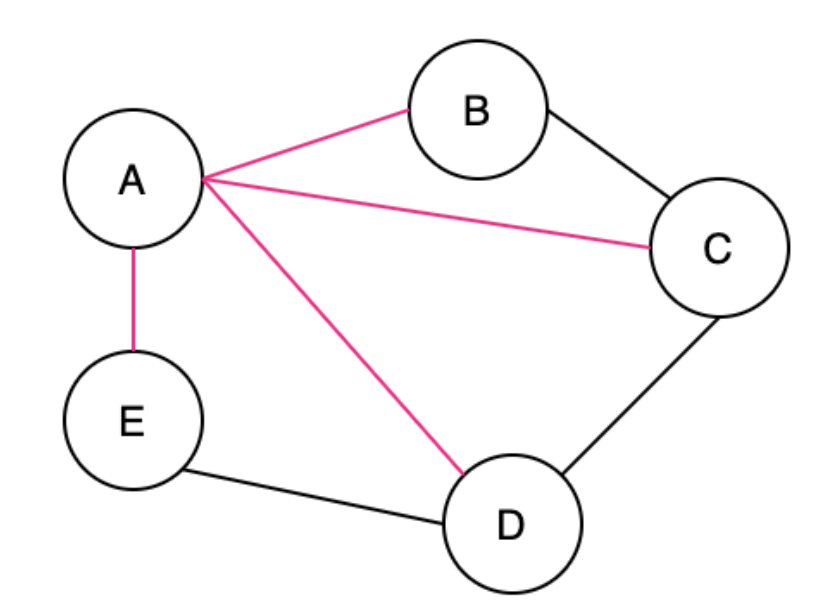
A Minimum Spanning Tree (MST) is when there are weights in a graph, you ideally can find the ST with the smallest total weight. An undirected graph can have multiple ST's and MST's

A cut in Graph Theory is a way to split up the Vertices and Edges in a Graph into 2 distinct sets, essentially cutting it to create 2 disjoint subsets. A crossing edge is an edge that connects a vertex in one set with a vertex in another set

Cut

So the cut property, which will help us run different algorithms, says for any cut $C$ of the graph $G$ , if the weight of an edge $E$ in a cut-set $C_s$ is strictly less than all other edges in $C_s$ , then $E$ belongs to all MST's of $G$

The proof above would rely on contradiction and goes something along the lines of "well if you didn't have that edge, $E$ in the MST, then you could add it and create a cycle that crosses the cut at least twice (first and newly added edge), and then if you removed the other Edge $E^`$ greater than it, it would result in a MST less than the original one"

MST algorithms are useful to find solutions to things like "min number of vertices to connect all points" similar to traveling salesman and finding paths between towns

Kruskal

Kruskal's Algorithm is for creating a Minimum Spanning Tree from a Weighted Undirected Graph. It uses sorting and UnionFind to solve for MST Kruskal's Algorithm will:

Sort all edges, taking $O(E \times log(E))$ time using a typical sorting algorithm
Create all connected components via UnionFind
Starting smallest, for each edge:
- Check if the vertices of the edge are in the same connected component, if not add the edge to the MST
  - Union find .union(x, y) function will return False if they're in same component, and True if they aren't. If they aren't in the same component it'll ensure that they are afterwards
- Adding an edge where 2 vertices are in the same connected component is equivalent to creating a cycle
Once you reach $V - 1$ $V - 1$ edges we've constructed our MST
- We know it's minimal because we're using the smallest of edges and greedily choosing at each point
- We know it's connected because we're only picking ones that connected disconnected components

Show Python Script

def kruskal_mst(vertices, edges):
    """
    Kruskal's MST Algorithm
    :param vertices: Number of vertices in the graph
    :param edges: List of edges (u, v, weight)
    :return: List of edges in the MST and the total weight
    """
    # Step 1: Sort edges by weight
    edges.sort(key=lambda x: x[2])

    # Step 2: Initialize Union-Find and MST
    uf = UnionFind(vertices)
    mst = []
    total_weight = 0

    # Step 3: Process edges
    for u, v, weight in edges:
        if uf.union(u, v):  # If u and v are not in the same component
            mst.append((u, v, weight))
            total_weight += weight

            # Stop if you have V - 1 edges in the MST
            if len(mst) == vertices - 1:
                break

    return mst, total_weight

Time Complexity	Space Complexity
$O(E \times log(E) + \alpha(V)) = O(E \times log(E))$	$O(V)$

Prim

Prim's Algorithm is another algorithm for creating a Minimum Spanning Tree from a Weighted Undirected Graph. It uses 2 sets to solve for MST

Prim's algorithm adds edges to a min-heap for all neighbors of a node. Essentially Prim's algorithm starts at an arbitrary node and performs DFS over all neighbors, adding the edge weight to the min-heap. It skips all visited nodes if it encounters them in the min heap, and will continuously add nodes to the MST via the first seen edge until it has $V-1$ edges

Show Python Script

def prim_mst(vertices, graph):
    """
    Prim's MST Algorithm
    :param vertices: Number of vertices in the graph
    :param graph: Adjacency list representation of the graph
    :return: List of edges in the MST and the total weight
    """
    # Initialize
    mst = []
    total_weight = 0
    visited = [False] * vertices
    min_heap = []

    # Start from arbitrary vertex
    visited[0] = True
    for neighbor, weight in graph[0]:
        heapq.heappush(min_heap, (weight, 0, neighbor))  # (weight, from, to)

    # Process the priority queue
    # This will start with smallest weighted edge that you found from 0
    while min_heap:
        weight, u, v = heapq.heappop(min_heap)

        if not visited[v]:
            # Add edge to MST
            visited[v] = True
            mst.append((u, v, weight))
            total_weight += weight

            # Add all edges from the new vertex to the heap
            for neighbor, edge_weight in graph[v]:
                if not visited[neighbor]:
                    heapq.heappush(min_heap, (edge_weight, v, neighbor))

    return mst, total_weight

Finding all the edges that connect the 2 sets is the majority of complexity here, and typically is solved using

Time Complexity	Space Complexity
$O(E \times log(V))$	$O(V)$

Shortest Path

Breadth First Search can help us find the shortest path between 2 nodes in an unweighted graph, but it can't help when the graph is weighted because there are so many more options! BFS in an unweighted scenario goes out one-by-one for each level, and so we know if we reach any node $N$ from our origin node $O$ , that we've found the shortest path, but in a weighted graph there may be a "longer" route over more edges that's actually shorter given weights

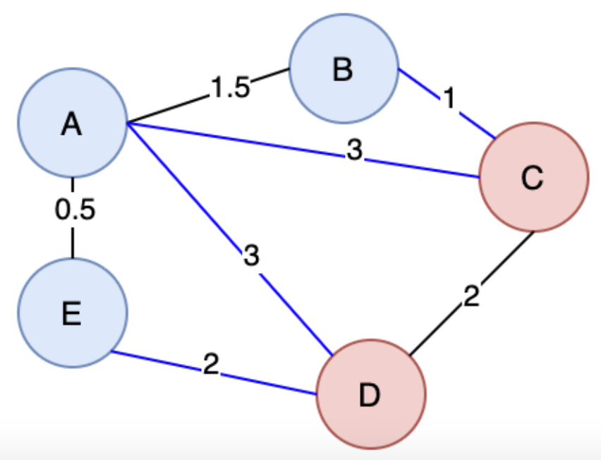
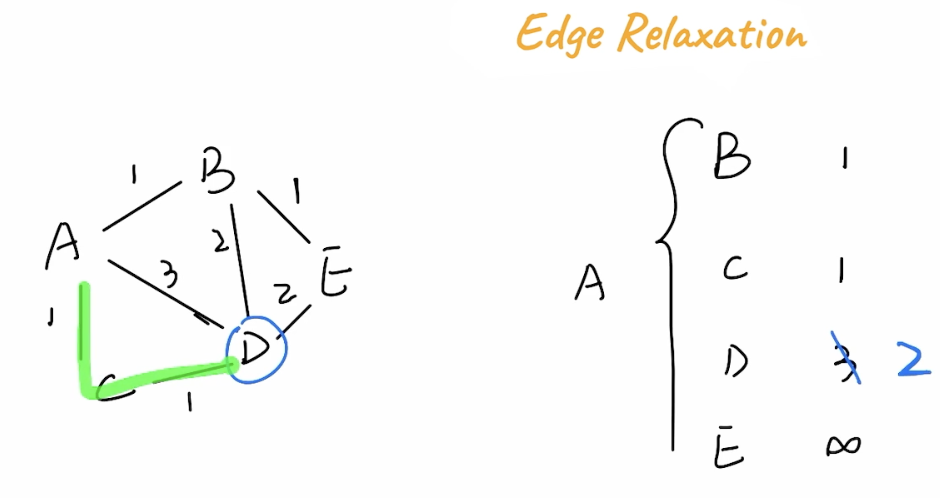
Edge Relaxation

The Edge Relaxation Property is the general property describing that although a path might take more hops, the weights on it might be smaller. In the below example A -> C -> D has a total weight of 2, while A -> D has a weight of 3 Edge Relaxation Example

Djikstra

Djikstra's Algorithm can help solve the shortest path problem for graphs with non-negative weights

It solves the shortest path problem for a single vertex, to all other vertices by utilizing a min heap:

Sets distance to +inf for all nodes, except the source node which is set to 0
Place source node with current distance of 0 into min heap
While the min heap has entries
- Find current node
- From that node, get the current node's weight plus the total weight to move to a destination node
- If this weight is less than what's been previously seen at the destination node, mark the destination node's weight as that
- Add to the min heap

You also showcase this problem in Pregel Graph Processing Docs - in most cases you can't hold an entire graph in memory, and we'll have it written to disk somewhere, and Pregel is a Graph Traversal SDK for distributed datasets using Spark

Djikstra's algorithm is greedy, and essentially starts from a central point u and expands outwards, continually getting the min from the seen vertices to find shortest path to other vertices, it uses a min-heap to continuously select the vertex with the smallest known distance

Hold the state of our source vertex to each other vertex in the graph, and you hold "previous vertex" and length information in this table which will help us traverse recursively if you needed to rebuild the path. you can lookup distance from source to any other vertex in $O(1)$ once it's complete, and then rebuilding path is at worst $O(E)$ because it might be a linked list, and building this data structure and traversing the graph resutls in us visiting each vertex and each node so it would be around $O(V + E)$ time complexity, but for each edge in a vertex you need to find the min vertex which is $O(log V)$ , therefore total time complexity is $O(V + E \times log(V))$ and $O(V)$ space (since you need to store visited node info)

Time Complexity	Space Complexity
$O((V + E) \times log(V))$	$O(V + E)$

Use cases:
- Network delay times from source to all sinks
- Traveling salesman that needs to cover all houses
- ...

Show Python Script

def dijkstra(graph, source):
    """
    Dijkstra's Algorithm to find the shortest path from a source to all other vertices.
    :param graph: Adjacency list representation of the graph {node: [(neighbor, weight), ...]}
    :param source: The starting vertex
    :return: A tuple (distances, previous_nodes)
             distances: Dictionary of shortest distances from the source to each vertex
             previous_nodes: Dictionary to reconstruct the shortest path
    """
    # Initialize distances and priority queue
    distances = {vertex: float('inf') for vertex in graph}
    # store distance from source to vertex
    distances[source] = 0
    # store the node we used to get to this vertex (to reconstruct path later)
    previous_nodes = {vertex: None for vertex in graph}
    min_heap = [(0, source)]  # (distance, vertex)

    while min_heap:
        # O(log V)
        current_distance, current_vertex = heapq.heappop(min_heap)

        # Skip if the current distance is not optimal
        #   if equal continue on to potentially find shorter
        #   paths for other nodes
        # This should only occur if this current vertex's weight
        #   here was added, say A ---10---B
        #   and a shorter route was found later such as
        #   A --3-- C --2-- B, which would have distances[B] = 5
        #   and this would then skip. If we didn't skip then
        #   it would use distances[B] = 10 below for neighbor
        #   values, which would be incorrect
        if current_distance > distances[current_vertex]:
            continue

        # Explore neighbors
        for neighbor, neighbor_weight in graph[current_vertex]:
            neighbor_distance = current_distance + neighbor_weight

            # If a shorter path is found
            if neighbor_distance < distances[neighbor]:
                distances[neighbor] = neighbor_distance
                previous_nodes[neighbor] = current_vertex
                # O(log V)
                heapq.heappush(min_heap, (neighbor_distance, neighbor))

    return distances, previous_nodes


def reconstruct_path(previous_nodes, target):
    """
    Reconstruct the shortest path from the source to the target.
    :param previous_nodes: Dictionary of previous nodes from Dijkstra's algorithm
    :param target: The target vertex
    :return: List of vertices representing the shortest path
    """
    path = []
    while target is not None:
        path.append(target)
        target = previous_nodes[target]
    return path[::-1]  # Reverse the path

Bellman-Ford

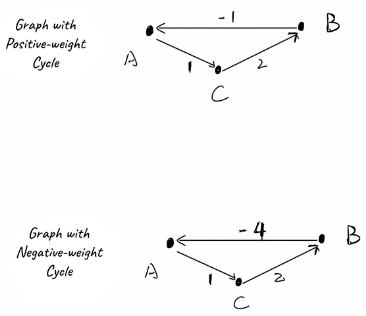
Bellman-Ford works for all graph types that are not negative cyclical - meaning even if there's a positive weight cycle, we are still able to find shortest path between 2 nodes

The official problem statement from competitive programming bellman ford is "Suppose that we are given a weighted directed graph $G$ with $n$ vertices and $m$ edges, and some specified vertex $v$ . You want to find the length of shortest paths from vertex $v$ to every other vertex."

2 theorem's that are used to get there:

"In a graph with no negative-weight cycles with $N$ $N$ vertices, the shortest path between any two vertices is at most $N-1$ $N - 1$ edges
- Even if the direct link between 2 nodes is not the shortest, if every weight is non-negative, then we can only add on more distance if we go over $N-1$
- If we do use $N-1$ we've "used all the weights", and so there's no way adding on more could result in less distance, as everything is non-negative
"In a graph with negative weight cycles there is no shortest path"
- We can continuously reduce distance in a cycle by looping around forever

Positive vs Negative Weight Cycle

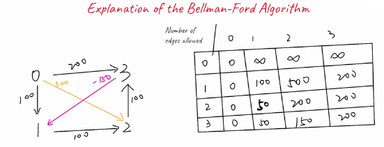
Using the two theorems above you can setup a table where rows are vertices $[1, ..., N-1]$ that represent the number of edges allows, and columns are the $[0, ... , N]$ vertices. We know it can only be up to $N-1$ . Bellman-Ford can't detect shortest path with negative weight cycles, but it can detect if there's a negative weight cycle, and then return early with impossible

Initiate tabel at [0, 0]
Go through each row which represents the number of edges allowed
- Utilize the row above to find the minimum distance to any of the potential neighbors
- For example [1, 3] represents distance of 200 which is using 1 row to get from source 0 to node 3, and then from 3 we can reach node 2 with weight -150 so we can add -150 + 200 = 50 < +inf

Bellman Ford DP Table

Can optimize this further by realizing it only needs to store the last row above, representing the shortest path from source if at most $K-1$ edges are used, or by using the current row which represents shortest path from source if at most $K$ edges are used

Bellman-Ford Implementation

Setup:

$n$ vertices and $m$ edges
There will be at most $n-1$ edges
Source vertex $v$
Initialize distance array $d[0, ... n-1]$ $d [0, ... n - 1]$
- This will hold the answer at the end for the shortest weighted total from $v$ to each $n-1$
- $d[v] = 0$ , and the rest will be inf at the start
At each step we only need to host the shortest distance seen so far for any node $x$ $x$ as $d[x]$ $d [x]$
- We loop over each edge in the graph $e = (x, y)$ having weight $c$ , and try to produce relaxation
- Relaxation is an attempt to improve $d[y]$ $d [y]$ using value $d[x] + c$ $d [x] + c$
  - In this way, we only need to host the shortest distance so far to $d[x]$
$n-1$ phases are sufficient to correctly calculate the lengths of all shortest paths in the graph (as long as there aren't any negative cycles) as unreachable vertices will remain inf

Show Python Script

# List of edges is an easier structure to utilize given we
#   have to loop over all edges in each iteration
def bellman_ford(self, n: int, v: int, edges: List[List[int]]) -> List[int]:
  # Edges = [ [from_x, to_y, weight] ]
  distances = [float("inf")] * n
  d[v] = 0
  for level in range(n-1):
    tmp = distances[:]

    for edge in edges:
      if distances[edge[0]] < float("inf"):
        tmp[edge[1]] = min(
          tmp[edge[1]],

          # we need to check based on currently known distances
          #   otherwise we may traverse a graph in a single iteration
          #   that's not supposed to be updated
          distances[edge[0]] + edge[2]
        )
    
    distances = tmp

So ultimately we're just tracking the min distance we've seen at any node and utilizing that plus any of it's outbound edges to calculate a min distance for another node

If we want to also retrieve the path we can store a previous_node lookup table similar to djikstra

Show Python Script

# List of edges is an easier structure to utilize given we
#   have to loop over all edges in each iteration
def bellman_ford(self, n: int, v: int, edges: List[List[int]]) -> List[int]:
  # Edges = [ [from_x, to_y, weight] ]
  distances = [float("inf")] * n
  d[v] = 0
  paths = [-1] * n

  for level in range(n-1):
    early_stop = True
    for edge in edges:
      if edge[0] < float("inf"):
        if distances[edge[1]] > distances[edge[0]] + edge[2]:
          early_stop = False
          paths[edge[1]] = edge[0]
          distances[edge[1]] = distances[edge[0]] + edge[2]
    
    # no work was done
    if early_stop:
      break
  
  # no path exists
  if d[v] == float("inf"):
    return(-1)
  
  resp = []
  target = v
  while target != -1:
    resp.append(target)
    # get previoous node
    target = paths[taret]

  return(resp[::-1])

Bellman-Ford With Negative Cycle

All of the above revolves around there being absolutely no possibility of a negative cycle, which isn't always true. If there is a negative cycle we can detect it in a few ways - the easiest one being if there's another potential relaxation after the $N-1$ cycle, then we're in a forever loop negative cycle and we should return immediately. In the presence of a negative cycle, and node in the same component should have a total distance of -inf as you could loop around forever in that negative cycle infinite times, and then go traverse to some reachable node

To implement negative cycle detection + negative cycle path retrieval we use neg_cycle_flg

If any edge can still be relaxed, i.e. distances[edge[1]] > distances[edge[0]] + c, then neg_cycle_flg is set to the destination node edge[0]
If we run all $N-1$ iterations, and then we're still able to relax something, it means there's a negative cycle
So we loop backwards $N$ times from current node to ensure we move back into the negative cycle on a node y
Then continuously reconstruct the path until we reach y again

Show Python Script

# List of edges is an easier structure to utilize given we
#   have to loop over all edges in each iteration
def bellman_ford(self, n: int, v: int, edges: List[List[int]]) -> List[int]:
  # Edges = [ [from_x, to_y, weight] ]
  distances = [float("inf")] * n
  d[v] = 0
  paths = [-1] * n

  # This is changed to n, which would allow another
  #   iteration to check for a relaxation possibility
  for level in range(n):
    early_stop = True
    neg_cycle_flg = -1

    for edge in edges:
      if edge[0] < float("inf"):
        if distances[edge[1]] > distances[edge[0]] + edge[2]:
          early_stop = False
          paths[edge[1]] = edge[0]
          distances[edge[1]] = distances[edge[0]] + edge[2]
          neg_cycle_flg = edge[1]
    
    # no work was done
    if early_stop:
      break
  
  # negative cycle detected
  if neg_cycle_flg != -1:

    # ensure y is in negative cycle
    #   following it back n times guarantees
    #   we end at a node in the cycle
    y = neg_cycle_flg
    for i in range(n):
      y = paths[y]
    
    bad_path = []
    curr = y
    while curr != y:
      bad_path.append(curr)
      curr = paths[curr]

Topological Sorting / Kahns Algorithm

Topological Sorting can help us traversing graphs when there are dependencies in directed acyclic graph's (DAGs), which is different from the above undirected weighted graphs

A key property is acyclic meaning there are no cycles in the graph! It wouldn't make sense if our prerequisites were required for our prerequisites!

Use cases:
- Course scheduling with pre-requisites
- Workflow DAGs
- ...

The main algorithm for this is Kahn's Algorithm where you will basically iterate over all vertexes that have indegree = 0, and do something with them, and then decrement their downstream vertexes. This ultimately creates "levels" where multiple classes or jobs could be ran at the same time, and once they're all done you should be ready for our downstream vertexes (decrement indegree)

The most common problem is the Dependent Course Problem where you need to build a DAG of pre-requisite courses and then figure out how many semesters it would take to complete all courses

Since you are only iterating over edges and vertexes and doing increment / decrement, our space and time complexities are $O(V + E)$

Time Complexity	Space Complexity
$O(V + E)$	$O(V + E)$

Show Python Script

    in_degree = {i: 0 for i in range(vertices)}
    adjacency_list = defaultdict(list)

    for u, v in edges:
        adjacency_list[u].append(v)
        in_degree[v] += 1

    # Step 2: Collect nodes with in-degree 0
    zero_in_degree = deque([node for node in in_degree if in_degree[node] == 0])

    # Step 3: Perform topological sort
    topo_order = []
    while zero_in_degree:
        current = zero_in_degree.popleft()
        topo_order.append(current)

        # Reduce in-degree of neighbors
        for neighbor in adjacency_list[current]:
            in_degree[neighbor] -= 1
            if in_degree[neighbor] == 0:
                zero_in_degree.append(neighbor)

    # If topo_order doesn't contain all vertices, there is a cycle
    if len(topo_order) != vertices:
        raise ValueError("The graph contains a cycle and cannot be topologically sorted.")

You can also utilize straight up DFS for topological sort in some dependency graph problems by utilizing the 3-color masking method. Ultimately this relates to tracking state along the call stack, and if something is currently in the stack (lookup in state = defaultdict(int) dict) with state = 1, then it's a loop as you'll eventually form a cycle

Leaves Of A Binary Tree also has implementations for DFS, better DFS, and topological sort (BFS)

state[u] = 1
for v in deps[u]:
    dfs(v)
state[u] = 2
order.append(u)

You need to do postorder traversal for this to work, as for any node you need to go completely explore all of the nodes it depends on - so you'll need some sort of dictionary like services_depends_on where each key is a specific node, and each item in the value list is another node that it will depend on. Once you go through all of those, and eventually add them to your order response, it'll be a topologically sorted array

Cycles In Directed Graph

Similar to cycles in an undirected graph, we have a few options for calculating cycles:

Can store visited / seen nodes along with some relationship as we traverse a graph in DFS. However, in a directed graph we also need to track if the node has been seen in this iteration, versus another iteration, and this is known as coloring
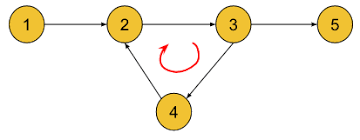
Can use topological sorting, and then if any nodes at the end have in-degree > 0, that means it's apart of a cycle
- In the below graph, the only in-degree = 0 would be node 1, after that there's nothing with that, and so there's a cycle

Cyclic Directed Graph

Show Stack Coloring Cycle DAG Python Script

def isCyclicHelper(self, node, graph, visitedArr, currStackArr):
  # this node is inside the current stack / loop
  if currStackArr[node]:
    return(True)

  # we've visited this node, but not in this stack / loop
  if visitedArr[node]:
    return(False)
  
  visitedArr[node] = True
  currStackArr[node] = True
  
  for neighbor in graph[node]:
    if self.isCyclicHelper(neighbor, graph, visitedArr, currStackArr):
      return(True)
  
  currStackArr[node] = False
  return(False)

def isCyclic(self, graph):
  n = len(graph)

  visited = [False] * n
  currStack = [False] * n

  for node in range(n):
    if not visited[node] and self.isCyclicHelper(node, graph, visited, currStack):
      return(True)
  
  return(False)

An easier to remember option, that also allows to slice out the cycle, and find many cycles, is doing white, grey, black coloring on a node

Show WGB Coloring Cycle DAG Python Script

def getCycles(self, graph):
  # graph is full adjacency list of fromNode: [toNodes]
  self.n = len(graph)
  self.color = {node: 0 for node in range(self.n)}
  self.path = []
  self.cycles = []

  for node in range(self.n):
    if self.color[node] == 0:
      self.dfs(graph, node)

  return(self.cycles)

def dfs(self, graph, node):
  self.color[node] = 1
  self.path.append(node)
  for neighbor in graph[node]:
    if self.color[neighbor] == 0:
      self.dfs(graph, neighbor)
    elif self.color[neighbor] == 1:
      idx = self.path.index(neighbor)
      self.cycles.append(self.path[idx : ] + [neighbor])
  
  # need to pop off for future cycles to not include
  self.path.pop()
  self.color[node] = 2

Advanced Graph Topics

Below topics are more around Graph Theory, random stuff from lectures, etc

Graph Types

Graphs can have a few different topological setups as well - including:

Multi-Relational: A graph that has more than one type of relationship between vertices
- In a social network we can have friend, family, coworker, etc..
  - Formally, a multi-relational graph is defined as $G = (V, T, E)$ where $T$ is a set of edge-types
- The adjacency matrix in this scenario would be a $3-D$ $3 - D$ matrix (a Tensor), where $A[n1, n2, type] = 1$ $A [n 1, n 2, t y p e] = 1$ if there's an edge of type type between n1 and n2
  - The tensor dimension here would be $V \times V \times T$
Multiplex: A graph where there are multiple types of edges between the same pair of vertices, and furthermore each edge has it's own weight
- It introduces intra-layer (within) and inter-layer (between)
  - Intra layer edges are edges that connect nodes for that layer type
  - Inter layer edges are routes that connect nodes across different layer types
- Using transportation network as an example, where nodes are cities and the types are transportation types (flight, rail, train, car, walk, etc...)
  - Intra layer edges represent getting between 2 citites using a single transportation type
  - Inter layer routes represent getting between 2 cities utilizing more than 1 transportation type

Sub Graph and Node Statistics

Graph statistics revolve around profiling graphs, sub-graphs, and other components by using various metrics and algorithms to understand their structure and properties - some are basic counting, some are combinatorics, and some are more advanced distributions. They answer questions about centrality, sparsity, density, connectivity, and other metrics

A common one to start off is cluster (sub-graph) density, and the intuition is finding the ratio of observed edges to possible edges within a cluster or sub-graph

$\text{possible connections} = \frac{n \cdot (n-1)}{2}$
$\text{observed connections} = e$
$\text{cluster density} = \frac{\text{observed connections}}{\text{possible connections}}$

The "hello world" of graph statistics is centrality utilizing the Florentine Families Dataset, which showcases relationships between families in Renaissance Florence, and typically should always have the Medici family as the most central node

To get to centrality and other metrics, there are some common statistics we'll define below:

Degree: The number of edges connected to a vertex
- In-Degree: Number of incoming edges to a vertex (for directed graphs)
- Out-Degree: Number of outgoing edges from a vertex (for directed graphs)
Degree Centrality: The number of edges connected to a vertex, normalized by the maximum possible degree
- If there are 8 nodes in a graph, and a specific node has 2 edges to 2 other nodes, it's degree centrality would be (\frac27)
Path Length: The number of edges in the shortest path between two vertices
Clustering Coefficient: A measure of the degree to which nodes in a graph tend to cluster together
- For a vertex, it's the ratio of the number of edges between its neighbors to the number of possible edges between those neighbors
- For the whole graph, it's the average clustering coefficient of all vertices
Betweenness Centrality: A measure of how often a node appears on the shortest paths between other nodes
- Betweenness shows how often a node lies on the shortest path between two other nodes, and these nodes can be considered "route hubs" of sorts
- Cincinnati is a good example used to illustrate betweenness centrality in transportation networks, no one ever stops there, everyone just drives through it
Eigenvector Centrality: A measure of a node's influence based on the influence of its neighbors
- Sum of centrality scores of neighbors
Closeness Centrality: A measure of how close a node is to all other nodes in the graph, based on the average shortest path length from the node to all other nodes
- Inverse of average shortest path length to all other nodes
- Gives information on how close a node is to all other nodes, and simply showcases what node, even if it's not as important, is closest to everything
Subgraph classifications and definitions:
- Closed Triangles: Sets of three nodes where each node is connected to the other two nodes
- Ego Graphs*: Subgraphs consisting of a focal node, and all the nodes that are connected to that focal node
  - Most likely is star shaped
- Motifs: Patterns of node connectivity that occur more than would be expected by chance
  - Basically a catch all for sub-graph patterns - closed triangles and ego graphs are specific motifs
Clustering Coefficient: Measures the proportion of closed triangles in a node's local neighborhood
- Can be used to find communities in a network, which help to show how clustered a node is
- $\frac{\text{# of triangles in a node's local neighborhood}}{\text{# of possible triangles in a node's local neighborhood}}$

Eigenvectors in Graphs

Seeing an Eigenvector scared me - they're actually utilized in Graph Theory to understand how certain graphs change as operations are performed on them

Eigenvectors can be used to find equilibrium points of graphs, which ultimately are points that aren't affected by any changes that are made to it

Graphs are just matrices, so eigenvectors help us understand their properties and behaviors - an adjacency matrix represents the connections between nodes, and therefore eigenvectors represent directions in which the graph can be transformed without changing its structure

An adjacency matrix can be seen as a transformation that acts on "node vectors", or functions defined on the graphs nodes

The intuition of an eigenvector on an adjacency matrix is that it allows us to find important nodes in a graph, where the eigenvector centrality of a node is proportional to the sum of the centralities of its neighbors

Some intuition from Reddit

Some definitions on GeeksForGeeks

Some Medium Articles

If we wanted to find a function below that essentially brings a node to the real numbers, we can use a vector with one entry for any node - i.e. a node vector $f(\text{node}) \rarr \mathbb{R}$

Backtracking a bit, this ends up relating to harmonic functions, which are function $f: \mathbb{R} \rarr \mathbb{R^2}$ that is always equal to it's average on circles - this means the function is always reverting towards it's average within some bounding box

The analogy of eigenvectors on graphs is a node vector so that each entry is always equal to the average of the entries of it's neighbors - i.e. within a small bounding box (neighbors), we want the eigenvector entries to always be equal to the average of it's neigbors. Therefore, if an eigenvector's value is large, we can see that it's node (the average of it's neighbors) means that node and it's neighbors must be a sort of critical central component

This node vector intuitively encodes some information about adjacency between nodes, and ultimately this encoded vector would have to be constant over each connected component of a graph (they're all neighbors)

Therefore, at the end, eigenvector centrality (eigencentrality) is a measure of the influence of a node in a network!

PageRank and Katz centrality are related concepts that build upon eigenvector centrality to rank nodes in a network, and they are natural variants of this eigencentrality

The $v^{\text{th}}$ component of the related eigenvector gives the relative centrality score of the vertex $v$ !

What can this help us with graph profiling:

Graph structure: Eigenvectors can reveal overall "sub-clusters" within a graph, and reveal if the entire graph is highly connected
Centrality measures: The eigenvector values are measure's of node importance that consider both the node's direct connections, and their neighboring node's
- Assigning higher scores to nodes that are connected to other highly connected central nodes
Network dynamics: Eigenvectors can be used to understand the stability or equilibrium of processes on the network, and can even help us find steady state distributions and feeback loops (similar to markov chains)
Community detection: Eigenvectors can be used in community detection algorithms to identify groups of nodes that have similar connectivity patternss

Proof / Math

For a given graph $G := (V, E)$ with $|V|$ vertices
$A = (a_v, t)$ $A = (a_{v}, t)$ is the adjacency matrix such that
- $a_{v, t} = 1$ if vertex $v$ is linked to vertex $t$
- 0 otherwise
$M(v)$ is a set of neighbors of vertex $v$

Then, the relative centrality score of a vertex $v$ can be defined as: $x_{v} = {\frac{1}{\lambda}} \sum_{t \in M(v)} x_t = {\frac{1}{\lambda}} \sum_{t \in G} a_{v,t} \cdot x_t$

Rearranging the above equation (somehow) you can get to vector notation where: $\bold{A}\bold{x} = \lambda \bold{x}$

There'll be many eigenvalues $\lambda$ for which a non-zero eigenvector solution exists, but extra conditions such as all entries in the eigenvector be non-negative (Perron-Frobenius) implies that only the greatest eigenvalue is considered for eigenvector centrality

The $v^{\text{th}}$ component of the related eigenvector gives the relative centrality score of the vertex $v$ !

Graph Statistics

Now they Sub-Graph and Node Statistics are covered above, there's a natural way to extend those to entire graphs

The typical proposal is to extract these metrics utilizing Graph Kernel Methods which are classes of ML algorithms that can be used to learn from data that's represented as a graph

Most graph kernel methods are proper ML algorithms, and so we'll define them further in Graph Neural Networks

Trees​

Binary Tree​

Complete and Perfect Binary Tree​

Binary Search Tree​

Insertion​

Deletion​

Self-Balancing Binary Search Tree​

AVL Tree​

Red Black Tree​

Segment Tree​

Prefix Sum​

Traversal Types​

Depth First Search​

Recursion Stack​

Breadth First Search​

Binary Search Tree​

Graphs​

Structuring​

Graph Traversal​

Graph Depth First Search​

Graph Breadth First Search​

Implicit Graphs​

Graph Problems and Advanced Data Structures​

Maze​

Connected Components​

Cycles + Connected Components In Undirected Graph​

Disjoint Set​

Terminologies​

Base Implementation​

Quick Find​

Quick Union​

Optimizations​

Union By Rank​

Path Compression​

Map Reduce Connected Componenets​

Minimum Spanning Tree​

Kruskal​

Prim​

Shortest Path​

Edge Relaxation​

Djikstra​

Bellman-Ford​

Bellman-Ford Implementation​

Bellman-Ford With Negative Cycle​

Topological Sorting / Kahns Algorithm​

Cycles In Directed Graph​

Advanced Graph Topics​

Graph Types​

Sub Graph and Node Statistics​

Eigenvectors in Graphs​

Proof / Math​

Graph Statistics​

Graphs In the Wild​

Storage​

Traversal / Compute​

Trees

Binary Tree

Complete and Perfect Binary Tree

Binary Search Tree

Insertion

Deletion

Self-Balancing Binary Search Tree

AVL Tree

Red Black Tree

Segment Tree

Prefix Sum

Traversal Types

Depth First Search

Recursion Stack

Breadth First Search

Binary Search Tree

Graphs

Structuring

Graph Traversal

Graph Depth First Search

Graph Breadth First Search

Implicit Graphs

Graph Problems and Advanced Data Structures

Maze

Connected Components

Cycles + Connected Components In Undirected Graph

Disjoint Set

Terminologies

Base Implementation

Quick Find

Quick Union

Optimizations

Union By Rank

Path Compression

Map Reduce Connected Componenets

Minimum Spanning Tree

Kruskal

Prim

Shortest Path

Edge Relaxation

Djikstra

Bellman-Ford

Bellman-Ford Implementation

Bellman-Ford With Negative Cycle

Topological Sorting / Kahns Algorithm

Cycles In Directed Graph

Advanced Graph Topics

Graph Types

Sub Graph and Node Statistics

Eigenvectors in Graphs

Proof / Math

Graph Statistics

Graphs In the Wild

Storage

Traversal / Compute